Course notes/Earth's energy balance

Note that you are not expected to memorize the terminology or formulae discuss here. They are included only to make it easier for you to connect what you're learning here with current issues in the news and what you might be learning in other courses and to make topics easier for you to look up if you find yourself interested in learning more. The primary purpose of these notes is to assist you in answering some of the WeBWorK problems that address Earth's energy balance.

Energy balance and equilibrium temperature of the earth

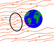
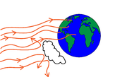
A simple model of energy balance and temperature on planet Earth is discussed in the course notes. It states that the energy input from the sun to Earth, called the insolation (not to be confused with insulation!), can be written as \begin{align} E_{in}=(1-a)S\pi r^2, \end{align} where $S$ measures the incoming radiation energy per unit area and $r$ is the radius of the earth so that $\pi r^2$ is the area of the profile of the earth exposed to the incoming radiation (see black circle in Figure 1). $a$ is the albedo (a number between 0 and 1) which represents the fraction of energy reflected so that $(1-a)$ is the fraction of energy absorbed by the planet (see Figure 2). $E_{in}$ has dimensions of energy per unit time.

Figure 1: Radiation coming from the sun delivers energy to Earth proportional to the area of the planet projected onto a plane perpendicular to the direction of the rays.

Figure 2: Some incoming radiation is reflected by the atmosphere and by the surface of the planet. This reflectiveness is represented in the equations by the albedo $a$.

Energy is lost from Earth into space by black-body radiation. The Stefan-Boltzmann Law describes the per-surface-area loss of energy from an object (like the earth) by black-body radiation as being proportional to the fourth power of the temperature of the object, $T$, measured in Kelvin. Some of the energy radiated away from the surface of the earth is reflected back in by the atmosphere (see Figure 3).

Figure 3: The planet gives off black body radiation but greenhouse gasses in the atmosphere reabsorbs some of it, only allowing a fraction of that radiation to escape. This escaping fraction is denoted by $\epsilon$, the emissivity.

The total energy that makes it out of the earth's atmosphere can be expressed as \begin{align} E_{out}=4\pi r^2 \epsilon \sigma T^4, \end{align} where $\epsilon$ is the emissivity of the Earth's atmosphere (the fraction of the outgoing radiation that actually escapes) and $\sigma$ is the Stefan-Bolzmann constant. $\sigma T^4$ is multiplied by the surface area of the planet, $4\pi r^2$, to get the rate of energy loss from the entire surface of the planet and that is multiplied by $\epsilon$ to get the fraction of the energy that escapes the atmosphere. If there were no greenhouse gasses in the atmosphere, $\epsilon$ would be 1. As greenhouse gasses accumulate in the atmosphere, $\epsilon$ decreases.

Figure 4 shows a schematic of the process.

Figure 4: A simplified picture of the earth's energy balance. Incoming radiation from the sun is partially reflected and partially absorbed (orange). Black body radiation is given off but only a fraction of it escapes the atmosphere (blue). The more greenhouse gasses that are present in the atmosphere, the more radiation is absorbed, allowing less to escape and thereby driving up temperature.

Let's explore what happens when there is an imbalance in the energy fluxes (i.e. the incoming and outgoing rates). When the incoming energy is greater than the outgoing energy, the energy of the planet increases. Most of this energy is converted into heat and therefore raises the planet's temperature (some goes into the atmosphere creating wind and some goes into plants via photosynthesis). On the other hand, when the incoming energy is less than the outgoing energy, the energy of the planet increases and so does the temperature. If these rates are equal, there is no change in temperature and we say the planet is at its equilibrium temperature.

It is critical to note that when the temperature increases, the outgoing energy also increases because it includes that $T^4$. This means that although excess incoming energy raises the temperature bringing the system closer to equilibrium, that temperature-increasing effect is self limiting because the outgoing energy increases at the same time. As the temperature gets closer to equilibrium, the rate of change drops ultimately driving the temperature to the equilibrium.

Similarly, excess outgoing energy lowers the temperature and hence lowers the outgoing energy itself which ultimately drives the system to equilibrium.

Finding an expression for $T_{eq}$ in terms of all the parameters is left as a WeBWorK exercise. Keep in mind that $T_{eq}$ will depend on $a$, $S$, $r$ $\sigma$ and $\epsilon$. If any of these parameters were to be changed, we could find a new value of $T_{eq}$ and thereby determine the influence of the change on the equilibrium temperature. Arguably more meaningful would be to calculate how much of a temperature change would occur as a result of a specific change in, say, the albedo $a$. We can express this as a ratio, the change in temperature per change in albedo: $$\frac{T_2-T_1}{a_2-a_1} = \frac{\Delta T_{eq}}{\Delta a}.$$ In fact, we can take the limit as $\Delta a \to 0$ and find $\frac{dT_{eq}}{da}$ which tells us, in an instantaneous sense, how quickly $T_{eq}$ changes as we change $a$. This quantity tells us how sensitive the global temperature is to changes in the albedo. A large value for $\frac{dT_{eq}}{da}$ means that $T_{eq}$ is sensitive to changes in $a$ whereas as small value of $\frac{dT_{eq}}{da}$ means $T_{eq}$ is insensitive to changes in $a$. Similarly, $\frac{dT_{eq}}{d\epsilon}$ tells us how sensitive $T_{eq}$ is to changes in emissivity.

Chain rule and the sensitivity of global temperature to CO$_2$ emissions

An issue of current interest is the influence of CO$_2$ emissions on global temperatures. Because this molecule is a good absorber of radiation, it decreases both the albedo and emissivity of the earth (which represent the fraction of incoming radiation reflected and outgoing radiation transmitted by the atmosphere respectively). To determine how much of an impact additional CO$_2$ would have on global temperature, we can calculate the sensitivity of $T_{eq}$ on the amount of greenhouse gas in the atmosphere.

As above, we can use derivatives to do this but our expression for $T_{eq}$ does not explicitly show the dependence on $G$. When you calculate the equilibrium temperature, you should get an expression that depends on both $a$ and $\epsilon$. Suppose for now that $a$ depends on $G$ but $\epsilon$ does not, nor do any other of the parameters ($S$, $\sigma$, $r$). We could write $T_{eq}$ using function notation as $T_{eq}(a)$ to emphasize the dependence on $a$. The equilibrium temperature can then be written as $T_{eq}(a(G))$. To find the sensitivity of $T_{eq}$ to changes in $G$, we would simply use the chain rule. Similarly, we could have ignored the dependence of $a$ on $G$ and calculated the sensitivity using a chain rule applied to $T_{eq}(\epsilon(G))$. Of course, neither of these two approaches is correct because $T_{eq}$ depends on both $a$ and $\epsilon$. We must therefore write down an expression for $T_{eq}$ that shows both dependencies and take the derivative of this more complicated expression. The calculation (which appears as a WeBWorK problem) requires several applications of the chain rule (two or three depending on how you count) and a quotient rule.

A differential equation for temperature

We can translate the verbal description of temperature change given above into a differential equation by recognizing first that the rate of heating is exactly determined by the difference between incoming and outgoing energy and second that the rate of heating is proportional to the rate of change of temperature where the constant of proportionality is called the heat capacity of the object ($C$), in this case of the earth. Putting those together, we get

\begin{align} C\frac{dT}{dt} = E_{in} - E_{out} = (1-a)S\pi r^2 - 4\pi r^2\sigma \epsilon T^4. \end{align}

Assuming that $a$, $S$, $r$ $\sigma$ and $\epsilon$ are all constant, we can draw the phase line for $T$. The steady state for this equation is exactly the equilibrium temperature calculated above. From the phase line, it should be clear that the equilibrium temperature is a stable steady state, consistent with the description given above.