Course notes/Fitting data - least squares

Describing the central tendency - an introduction to best-fit analysis

Imagine you have a data set from an experiment consisting of $n$ numbers, which we label $x_i, \ i=1...n$. If the quantity being measured was fairly consistent from measurement to measurement, you might expect it to be possible to find a single number that captures the essence of the entire experiment, a kind of summary number. The concept we're dealing with here is referred to as the central tendency. The most commonly used number that capture the notion of central tendency is the mean. Although you may be familiar with the mean, you might not know where it comes from. Here, we'll start with a discussion of how the mean arise from a formal "best-fit analysis" and then generalize the idea of a best-fit analysis to more complicated situations. The more complicated cases are "linear fit without intercept" and "linear fit with intercept". These are sometimes referred to as linear regression and when carried out using the sum of squared residuals (see below for details) might also be referred to as linear least squares.

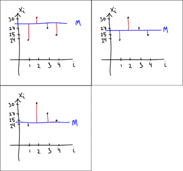
Let's try to find a number $M$ that simultaneous comes as close as possible to all the numbers in the data set. How do we formalize this idea of being as close as possible to an entire set of numbers? One approach would be to pick a value for $M$ that makes the sum of the distances as small as possible: $$\sum_{i=1}^n (x_i-M) = (x_1-M)+(x_2-M)+(x_3-M)+\cdots+(x_n-M)$$ where the notation $\sum_{i=1}^n c_i$ just means add up all the $c$ values, i.e. $\sum_{i=1}^n c_i = c_1+c_2+\cdots+c_n$. The individual quantities $r_i=x_i-M$ are called the residuals. Unfortunately, this expression simply keeps decreasing as you make $M$ larger. We need to make sure we get a positive contribution for each distance which is not the case for the sum of the residuals as above. There are two obvious ways that we can fix this problem: $$f(M)=\sum_{i=1}^n (x_i-M)^2= (x_1-M)^2+(x_2-M)^2+(x_3-M)^2+\cdots+(x_n-M)^2$$ and $$g(M)=\sum_{i=1}^n |x_i-M|= |x_1-M|+|x_2-M|+|x_3-M|+\cdots+|x_n-M|.$$ Both are good approaches and lead to numbers that describe the central tendency, albeit in different ways. Let's start with $f(M)$ which is called the sum of squared residuals (SSR). Notice that because the $x_i$ are just fixed numbers from your experiment, this expression is a function of the variable $M$. We're interested in finding the value of $M$ that returns the smallest value $f(M)$. This value is called the minimizer of the sum of squared residuals. This approach (minimizing the SSR) is referred to as the method of least squares. Let's look at an example.

Example

Suppose your data set consists of the numbers $\{24, 30, 27, 25\}$, plotted against their order in the list in Figure 1. In this case, \begin{align} f(M)=&(24-M)^2+(30-M)^2+(27-M)^2+(25-M)^2 \\ =& M^2 -2\times24M + 24^2 + M^2 -2\times30M + 30^2 + M^2 -2\times27M + 27^2 +M^2 -2\times25M + 25^2\\ =& 4M^2 -2(24 +30 + 27 +25)M + 24^2 + 30^2 + 27^2 + 25^2 . \end{align}

Figure 1 Residuals (in red) associated with three different possible fits (blue). Decide for yourself which on you think has the smallest sum of squared residuals.

This means the function we're trying to minimize ($f(M)$) is actually a quadratic. To find the minimum, we need only take a derivative and find the zeros: $$f'(M) = 2\times4M -2(24 +30 + 27 +25).$$ Solving for the zero of $f'$, we find $M=(24 +30 + 27 +25)/4$ which is precisely what's commonly called the average and more formally called the arithmetic mean or simply the mean.

In fact, this result is true in general. For a data set $x_i, \ i=1...n$, the mean of these values, $\bar{x}=\frac{1}{n}\sum_{i=1}^n x_i$, is the minimizer of the sum of squared residuals.

Another quantity that describes the central tendency

What happens if you minimize $g(M)$ instead? Because $g(M)$ is not differentiable at all points (it has corners where the derivative is not defined), we can't use calculus to find the minimizer. Graph it instead and see if you can figure out what other commonly used measure of central tendency minimizes it.

Statistical models

The mean is a simple example of a statistical model. A statistical model is a function that provides a good approximation to a set of data. In the case of the mean, the function is a constant. For data sets in which there is an apparent relationship between two variables (say $x$ and $y$), more complicated models can be used. For example, if the relationship between the variables in the data set appears to be linear, you might consider a linear model. There are two types of linear models, one with zero y-intercept and one with non-zero y-intercept. In practice, linear models with zero y-intercept are rarely used but they are simpler to analyze so we include them here as a introduction to the more complicated case of linear models with non-zero y-intercept.

Linear fit without intercept

Suppose we have another data set consisting of pairs of numbers $(x_i, y_i)$. Instead of just a number that approximates the x values or the y values, we want to find line that comes as close as possible to all the points simultaneously. For two points this is no problem. But what about three or more?

Example - concrete

Consider the data set consisting of the three points (1,2), (2,3) and (3,3) where the x coordinate represents the surface area of a leaf and the y coordinate represents the rate of photosynthesis. Your hypothesis is that the photosynthesis rate is linearly proportional to the surface area so $y=ax$. Note that this model has the very reasonable property that a leaf with zero surface area (not really a leaf at all) does not carry out photosynthesis at all. Mathematically, this means the line will definitely go through the origin. We now need to figure out how to make sure the line gets as close as possible to all three of the points in the data set as well. Clearly, there is no way we will be able to fit our line through all of these points (how do we know this?). Instead, we take a similar approach of minimizing residuals. In this case, the residuals are $r_i=y_i-ax_i$ and represents the vertical distance between each point and the line $y=ax$. We want to find the value of $a$ that minimizes the sum of squared residuals. We define the sum-of-squared-residuals function $$f(a)=(2-a)^2+(3-2a)^2+(3-3a)^2 = 14a^2-34a+22.$$ To find the minimum, we set the derivative equal to zero and solve for $a$: $$f'(a)=28a-34 =0$$ giving us $a=17/14$.

[Add plot].

Example - abstract

Let's repeat that with arbitrary data $(x_i,y_i)$ for i=1,2,3. \begin{align} f(a)=&(y_1-ax_1)^2+(y_2-ax_2)^2+(y_3-ax_3)^2\\ =& y_1^2 -2ax_1y_1 +a^2x_1^2 +y_2^2 -2ax_2y_2 +a^2x_2^2 + y_3^2 -2ax_3y_3 +a^2x_3^2\\ =& y_1^2+y_2^2+y_3^2 -2(x_1y_1 +x_2y_2 +x_3y_3)a + (x_1^2+x_2^2+x_3^2)a^2.\\ \end{align} Taking the derivative, we get $$f'(a) = 2(x_1^2+x_2^2+x_3^2) a - 2(x_1y_1 +x_2y_2 +x_3y_3).$$

Figure 2 Residuals (in red) associated with three different possible fits (blue). Decide for yourself which on you think has the smallest sum of squared residuals.

The critical point is at $$a=\frac{x_1y_1 +x_2y_2 +x_3y_3}{x_1^2+x_2^2+x_3^2}.$$ To see that it's a minimum, you can find the second derivative and you can see you'll end up with a positive constant $2(x_1^2+x_2^2+x_3^2)$.

General case

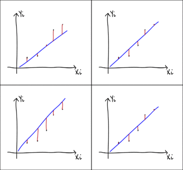
Here we state the result for the case of $n$ data points $(x_i, y_i)$ where $i=1,2,3\cdots n $ by analogy with the abstract three point case above. An example data set is plotted in Figure 2. The sum of squared residuals is $\sum_{i=1}^n (y_i-ax_i)^2$ and the value of $a$ that minimizes this quantity is $$a=\frac{\sum_{i=1}^n (x_iy_i)}{\sum_{i=1}^n x_i^2}.$$

Linear fit with intercept

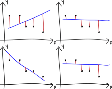
The more common form of linear fitting is to assume that the data can be described by a linear relationship of the form $y=ax+b$. Consider a general data set of coordinates $(x_i, y_i)$ where the points do not seem to line up well with the origin (see Figure 3). In this setting, the residuals are the quantities $r_i=y_i-ax_i-b$.

The sum of squared residuals is $f(a,b)=\sum_{i=1}^n (y_i-ax_i-b)^2$. In this case, there are two independent variables so the analysis requires multivariable calculus but the approach is essentially the same and the result is only a bit more complicated. The values of $a$ and $b$ that minimize the sum of squared residuals are

Figure 3 Residuals (in red) associated with three different possible fits (blue). Decide for yourself which on you think has the smallest sum of squared residuals.

$$a= \frac{P_{avg} - \bar{x}\bar{y}}{X^2_{avg}-\bar{x}^2}$$ and $$b = \bar{y} - a \bar{x}$$ where $$\bar{x}=\frac{1}{n}\sum_{i=1}^nx_i$$ (the average $x$ value), $$\bar{y}=\frac{1}{n}\sum_{i=1}^ny_i$$ (the average $y$ value), $$P_{avg}=\frac 1n \sum_{i=1}^{n}{x_{i}y_{i}} $$ (the average product of $x$ and $y$) and $$X^2_{avg}=\frac1n\sum_{i=1}^{n}\left({x_{i}^2}\right)$$ (the average value of the $x$ component squared).

Example

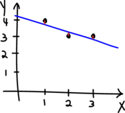
Let's find the line that best fits the data points (1,4), (2,3) and (3,3). The equation of the line will be $y=ax+b$ and we need to find the $a$ and $b$ values. I'll start by calculating all the necessary pieces and then assemble them into the formulae above. $$\bar{x}=\frac{1}{n}\sum_{i=1}^nx_i = \frac13(1+2+3)=2$$ $$\bar{y}=\frac{1}{n}\sum_{i=1}^ny_i = \frac13(4+3+3) = \frac{10}{3}$$ $$P_{avg}=\frac 1n \sum_{i=1}^{n}{x_{i}y_{i}} = \frac13(1 \times 4+ 2 \times 3 + 3 \times 3) = \frac13(4+6+9) = \frac{19}{3} $$ and

Figure 4 The data points (1,4), (2,3) and (3,3) and the line $y=-\frac{1}{2} x + \frac{13}{3}$ which is the best fit in the sense of linear least squares.

$$X^2_{avg}=\frac1n\sum_{i=1}^{n}\left({x_{i}^2}\right) = \frac13(1+4+9) = \frac{14}{3}.$$ Plugging these into the formulae for $a$ and $b$, we get $$a= \frac{P_{avg} - \bar{x}\bar{y}}{X^2_{avg}-\bar{x}^2} = \frac{\frac{19}{3} - \frac{20}{3}}{\frac{14}{3}-4} = \frac{19-20}{14-12} = \frac{-1}{2}$$ and $$b = \bar{y} - a \bar{x} = \frac{10}{3} - \frac{-1}{2} 2 = \frac{10}{3} + 1 = \frac{13}{3}.$$ So the best-fit line in the sense of least squares is $$y=-\frac{1}{2} x + \frac{13}{3}.$$

The sum of squared residuals for this line is $$f(a,b)=\sum_{i=1}^n (y_i-ax_i-b)^2.$$ For the best fit line we found above, $$ f\left(-\frac{1}{2},\frac{13}{3}\right)= \left(4+\frac{1}{2}\times 1 - \frac{13}{3}\right)^2 + \left(3+\frac{1}{2}\times 2 - \frac{13}{3}\right)^2 +\left(3+\frac{1}{2}\times 3 - \frac{13}{3}\right)^2= \frac{1}{6}.$$ If you were to try any other values of $a$ and $b$, you would get a larger value for f(a,b).